Fleet electrification financial models in Australia fall into two broad categories. There are the simple ones, fuel cost saving minus vehicle premium, payback in X years, that are directionally useful but too coarse to support a board-level investment decision. And there are the ones that exist inside government tender responses and research papers, which are thorough but inaccessible to fleet finance teams working under time pressure.
What’s missing is a practical, ten-year total cost of ownership framework that a CFO or fleet director can apply to their own operation using data they already have. This article provides that framework. It covers every cost category that matters, energy, maintenance, infrastructure, depreciation, financing, residual value, and explains how to model each one for a specific fleet rather than an industry average.
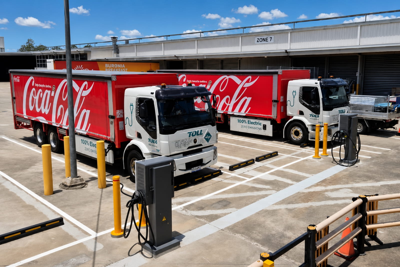
The framework draws on financial modelling from EVSE’s fleet electrification projects, including Toll Group’s Project TruckVolt and the CJD Equipment deployment, and is designed to produce the kind of analysis that supports a real investment decision rather than a policy discussion.
The Cost Categories That Matter
A complete ten-year fleet electrification model covers six cost categories. Most abbreviated models only capture two or three. The ones that get missed are often the ones that most significantly affect the answer.
1. Energy Costs
Energy is the most straightforward saving and the one most models capture correctly. The saving per kilometre between diesel and electricity in Australia is significant and relatively stable: diesel at approximately $2.20 to $2.40 per litre and commercial fleet consumption of 28 to 35 litres per 100km for heavy rigids produces a fuel cost of $0.62 to $0.84 per kilometre. Electric equivalents at a commercial off-peak tariff of $0.18 to $0.24 per kWh and consumption of 1.8 to 2.4 kWh per kilometre produce an energy cost of $0.32 to $0.58 per kilometre.
The spread, $0.10 to $0.46 per kilometre depending on vehicle type, diesel price, and electricity tariff, is the raw energy saving. For a heavy rigid covering 100,000km per year, this is $10,000 to $46,000 per vehicle per year. For a fleet of twenty vehicles, $200,000 to $920,000 annually.
The modelling nuance most teams miss: not all commercial charging occurs at off-peak tariffs. Vehicles that can’t be charged overnight due to operational patterns, or depots where the load management system isn’t correctly configured to shift load to off-peak windows, will incur shoulder or peak tariff rates. The model should use the realistic blended tariff for the specific fleet, not the best-case off-peak rate.
| Heavy rigid diesel fuel cost per km |
$0.62, $0.84 |
| Electric heavy rigid energy cost per km |
$0.32, $0.58 |
| Saving per km (range) |
$0.10, $0.46 |
| Annual saving: 20 vehicles at 100,000km each |
$200,000 to $920,000 |
| Model assumption to check |
Blended tariff vs off-peak rate |
2. Maintenance Costs
Maintenance cost reduction is the second-largest financial driver and the one most commonly under-modelled. The absence of engine oil changes, transmission fluid, exhaust aftertreatment (DPF, AdBlue), timing belts, and fuel injection systems removes cost items that represent $6,000 to $12,000 per heavy vehicle per year under a diesel maintenance regime.
Offset against this are new maintenance cost categories for electric drivetrains: battery health monitoring, cooling system maintenance, and software updates. These typically run to $1,500 to $3,000 per vehicle per year, producing a net maintenance saving of $4,500 to $9,000 per vehicle annually.
The ten-year cumulative maintenance saving for a fleet of twenty heavy vehicles is therefore $900,000 to $1,800,000, a figure that materially improves the overall investment case even before accounting for energy savings.
3. Infrastructure Costs
Infrastructure is the cost category that most significantly varies between projects and the one that undermines financial models most frequently. The range between a simple switchboard upgrade and a dedicated high-voltage substation can be $200,000 to $2,000,000 or more, and which end of that range applies to a specific depot depends entirely on site assessment data.
A model that uses a generic infrastructure assumption, or worse, ignores infrastructure costs and models only vehicle costs, will produce a payback period that bears no relationship to reality for many operators. The correct approach is to commission a site assessment as part of the modelling process, so the infrastructure cost input is a known figure rather than an assumption.
| AC charger installation (simple site, per unit) |
$1,500 to $4,000 |
| AC charger installation (complex infrastructure, per unit) |
$5,000 to $15,000 |
| Switchboard upgrade (if required) |
$8,000 to $45,000 |
| DNSP network augmentation |
$50,000 to $500,000+ |
| Dedicated HV substation |
$500,000 to $2,000,000+ |
| Load management software (annual, fleet of 20) |
$15,000 to $40,000 |
| Recommended approach |
Site assessment before modelling infrastructure |
4. Vehicle Depreciation and Residual Value
Electric heavy vehicles carry a purchase price premium of approximately 50 to 100 percent over diesel equivalents at current market prices. Over a ten-year model period, the depreciation of a vehicle worth $450,000 instead of $250,000 is a real cost, additional depreciation of approximately $20,000 per vehicle per year, or $400,000 for a fleet of twenty over ten years.
The offsetting factor is residual value uncertainty. Battery technology is improving rapidly and vehicle prices are falling. A diesel vehicle bought today has a well-understood residual value curve. An electric vehicle bought today has greater residual value uncertainty in both directions, the battery degradation profile affects resale value, but improving technology may also mean replacement battery packs become available at lower cost, sustaining vehicle value.
The conservative modelling approach is to assume zero residual value advantage for the electric vehicle over the diesel equivalent, i.e. the price premium is not recovered at resale. This is likely overly conservative given current trends, but it produces the most defensible investment case.
5. Financing Costs
The vehicle premium creates a financing cost if the fleet is acquired through debt or lease structures. An additional $200,000 per vehicle financed at 6.5% over seven years adds approximately $3,000 per vehicle per year in additional interest cost, $60,000 annually for a twenty-vehicle fleet. Over ten years, this represents $600,000 in additional financing cost that the energy and maintenance savings need to offset.
The financing equation changes materially with CEFC-backed concessional debt. A rate reduction of 0.75 to 1.0 percentage points on the vehicle acquisition finance reduces the total financing cost by $75,000 to $100,000 over seven years for a twenty-vehicle fleet. This is not a trivial adjustment to the model, and it’s one that well-prepared procurement teams will have explored before reaching the CFO presentation stage.
6. Grant Income
Government grant income for eligible fleet electrification projects is a real cash flow item, not a theoretical benefit. ARENA grant funding for projects meeting the scale and innovation criteria can offset 20 to 40 percent of infrastructure and project costs. State-level programs provide additional support that varies by jurisdiction and program availability.
The challenge in modelling grant income is the conditionality: grants are competitive, milestone-based, and subject to program availability at the time of application. A model that assumes grant income but hasn’t yet applied, or that assumes a grant quantum without confirmed approval, overstates the investment case. The conservative approach is to model grant income separately, show the base case without it, and show the grant-adjusted case as an upside scenario.
The 10-Year Model: Worked Example
The following is a simplified ten-year total cost of ownership model for a fleet of twenty heavy rigid vehicles, comparing diesel continuation against electrification. Figures use mid-range assumptions for all inputs.
| Fleet size |
20 heavy rigid vehicles |
| Annual kilometres per vehicle |
100,000km |
| Model period |
10 years |
DIESEL, 10-year total cost
| Vehicle acquisition (20 x $250,000) |
$5,000,000 |
| Fuel (20 vehicles, 100,000km, $0.73/km avg) |
$14,600,000 |
| Maintenance ($25,000/vehicle/year) |
$5,000,000 |
| Total diesel 10-year cost |
$24,600,000 |
ELECTRIC, 10-year total cost
| Vehicle acquisition (20 x $420,000) |
$8,400,000 |
| Charging infrastructure (mid-range depot) |
$800,000 |
| Energy (20 vehicles, 100,000km, $0.45/km avg) |
$9,000,000 |
| Maintenance ($16,000/vehicle/year) |
$3,200,000 |
| ALM software ($25,000/year) |
$250,000 |
| Total electric 10-year cost |
$21,650,000 |
| 10-year saving (electric vs diesel) |
$2,950,000 |
| Break-even point (approximate) |
Year 6 to 7 |
| Grant-adjusted break-even (30% infra grant) |
Year 5 to 6 |
Sensitivity note: The break-even point is most sensitive to infrastructure cost and annual kilometres. A depot requiring a $2M substation instead of $800K in infrastructure shifts break-even to Year 8 to 9. A fleet averaging 130,000km per vehicle per year instead of 100,000km shifts it to Year 5. Know your site and know your utilisation before presenting the model to a board.
The Variables That Move the Model Most
Infrastructure Cost: The Biggest Swing Factor
The difference between a $200,000 infrastructure project and a $2,000,000 one is the difference between a six-year and a twelve-year payback. This single variable has more effect on the investment case than fuel price assumptions, vehicle price trends, or maintenance cost estimates. Site assessment is the only way to know which end of the range applies to a specific depot. It should be the first expenditure in any serious electrification feasibility process.
Fleet Utilisation: The Multiplier
Every additional kilometre a vehicle travels increases the annual energy saving. A fleet that averages 120,000km per vehicle per year instead of 100,000km sees the ten-year energy saving increase by 20 percent. High-utilisation fleets, those running multiple shifts, long routes, or interstate operations, produce the strongest investment cases for electrification. Low-utilisation fleets, those with irregular operations or significant downtime, produce weaker ones.
Electricity Tariff: The Ongoing Lever
The model’s energy cost assumptions are based on commercial tariffs available today. Several variables can improve this figure over the model period: solar generation at the depot reduces the volume of grid energy purchased; battery storage shifts more charging to off-peak windows; TOU tariff optimisation through the load management system maximises the proportion of charging in the cheapest available periods. Each of these is worth modelling separately as a value-add scenario rather than baking optimistic assumptions into the base case.
Presenting the Model to the Board
A board-ready ten-year fleet electrification model should present three scenarios: conservative (higher infrastructure cost, current utilisation, no grants), base (site-assessed infrastructure cost, actual fleet data, no grants), and optimistic (grant income included, tariff optimisation, utilisation growth). The board needs to understand the conditions under which each scenario applies, not just the numbers.
Two additional elements strengthen the board presentation significantly. First, a sensitivity table showing how the break-even year changes with infrastructure cost and annual kilometres, this demonstrates that you understand the model’s key uncertainties and have quantified them. Second, a cash flow chart showing the cumulative cost of each scenario over ten years, which makes the crossover point visual and immediate.
The organisations that get fleet electrification investment approved at board level are not the ones with the most optimistic models. They’re the ones with the most credible ones, where every assumption is identified and justified, the sensitivity analysis is honest, and the downside case still produces a positive return over the model period.
Fleet electrification is not yet the obvious financial choice for every Australian transport operator. For high-utilisation fleets with accessible depot infrastructure and access to off-peak charging, it’s already a strong case. For lower-utilisation fleets or those facing significant infrastructure costs, the case depends on grant availability and longer-term fuel price assumptions. The model in this article is designed to show which situation a specific operator is in, not to produce a predetermined answer.
-
Job Title - Co-Founder, EVSE Australia
11 years of EV charging deployment history
EV specialist, ev driver, member of AFMA, AEVA, EV Council, HVIA
Sam Korkees is the Co-Founder of EVSE Australia, a leading provider of electric vehicle (EV) charging infrastructure and solutions. Since co-founding the company in 2014 alongside Brendan Wheeler, Sam has played a pivotal role in scaling EVSE from an early-stage startup into a nationally recognised leader in EV charging.
EVSE has delivered some of the country's largest EV fleet and depot charging deployments, supporting the electrification of commercial fleets, logistics operations, and government assets. The company is also recognised as a leader in public charging infrastructure, with extensive experience in the rollout of fast and ultra-fast DC charging networks nationwide.
Sam works closely with government, utilities, and enterprise clients to design and implement scalable, future-ready charging solutions, helping accelerate the adoption of EVs across Australia.
Credentials: 11 years of EV charging deployment history, EV specialist, EV driver, member of AFMA, AEVA, EV Council, HVIA